
Semanticity Classification with
EEG Artifact Removal with ATAR and Tuning
![]()
In this notebook, we demonstrate, how to apply ATAR algorithm built in spkit, whcih is combined with phyaat library now. The objective of including ATAR with phyaat is to make an easy to apply on phyaat dataset to quickly built a model for prediction task
We will only focus on one task - semanticity Classification and demonstrate the tuning part of ATAR and how that improve the performance. We will be extracting same spectral features that we have been using in other notebooks and examples, specifically 6 rhythmic features - total power in 6 frequency bands, namely, Delta (0.5-4 Hz), Theta (4-8 Hz), Alpha (8-14 Hz), Beta (14-30 Hz), Low Gamma (30-47 Hz), and High Gamma (47-64 Hz). For preprocessing, we filter EEG first with 0.5 Hz highpass and 24 Hz lowpass filter then remove Artifact with ATAR based approach.
Execute with ![]()
Table of Contents
import numpy as np
import pandas as pd
import matplotlib.pyplot as plt
#!pip install phyaat  # if not installed yet

import phyaat as ph
print('Version :' ,ph.__version__)
Version : 0.0.3
Download and Load a subject
# Download dataset of one subject only (subject=1)
# To download data of all the subjects use subject =-1 or for specify for one e.g.subject=10

dirPath = ph.download_data(baseDir='../PhyAAt/data/', subject=10,verbose=0,overwrite=False)
| 100%[ | ][##################################################] S10 |
baseDir='../PhyAAt/data/' # or dirPath return path from above

#returns a dictionary containing file names of all the subjects available in baseDir
SubID = ph.ReadFilesPath(baseDir)

#check files of subject=1
SubID[10]
Total Subjects : 3
{‘sigFile’: ‘../PhyAAt/data/phyaat_dataset/Signals/S10/S10_Signals.csv’, ‘txtFile’: ‘../PhyAAt/data/phyaat_dataset/Signals/S10/S10_Textscore.csv’}
Highpass and lowpass filtering
# Create a Subj holding dataset of subject=1

Subj = ph.Subject(SubID[10])

#filtering with highpass filter of cutoff frequency 0.5Hz and lowpass with 24 Hz (no reason why)

Subj.filter_EEG(band =[0.5],btype='highpass',method='SOS',order=5)
Subj.filter_EEG(band =[24],btype='lowpass',method='SOS',order=5)
ch_names = list(Subj.rawData['D'])[1:15]
fs=128
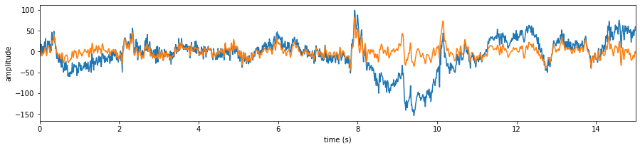
Let’s check the signals
# Let's check the signals

X0 = Subj.getEEG(useRaw=True).to_numpy()[fs*20:fs*35,1]
X1 = Subj.getEEG(useRaw=False).to_numpy()[fs*20:fs*35,1]
t = np.arange(len(X0))/fs

plt.figure(figsize=(15,3))
plt.plot(t,X0)
plt.plot(t,X1)
plt.xlim([t[0],t[-1]])
plt.xlabel('time (s)')
plt.ylabel('amplitude')
plt.show()

ATAR Algorithm
help(Subj.correct)
Help on method correct in module phyaat.ProcessingLib:
correct(method=’ICA’, Corr=0.8, KurThr=2, ICAMed=’extended-infomax’, AF_ch_index=[0, 13], F_ch_index=[1, 2, 11, 12], wv=’db3’, thr_method=’ipr’, IPR=[25, 75], beta=0.1, k1=10, k2=100, est_wmax=100, theta_a=inf, bf=2, gf=0.8, OptMode=’soft’, wpd_mode=’symmetric’, wpd_maxlevel=None, factor=1.0, packetwise=False, WPD=True, lvl=[], fs=128.0, use_joblib=False, winsize=128, hopesize=None, verbose=0, window=[‘hamming’, True], winMeth=’custom’, useRaw=False) method of phyaat.ProcessingLib.Subject instance
Remove Artifacts from EEG using  ATAR Algorithm or ICA
------------------------------------------------------
method: 'ATAR' 'ICA',
=====================

# For ICA  parameters (5)
---------------------------
ICAMed : (default='extended-infomax') ['fastICA','infomax','extended-infomax','picard']
KurThr : (default=2) threshold on kurtosis to eliminate artifact, ICA component with kurtosis above threshold are removed.
Corr   : (default=0.8), correlation threshold, above which ica components are removed.

Details:
ICA based approach uses three criteria
 - (1) Kurtosis based artifacts - mostly for motion artifacts
 - (2) Correlation Based Index (CBI) for eye movement artifacts
 - (3) Correlation of any independent component with many EEG channels

To remove Eye blink artifact, a correlation of ICs are computed with AF and F

For case of 14-channels Emotiv Epoc
ch_names = ['AF3','F7
PreProntal Channels =['AF3','AF4'], Fronatal Channels = ['F7','F3','F4','F8']
AF_ch_index =[0,13] :  (AF - First Layer of electrodes towards frontal lobe)
F_ch_index =[1,2,11,12] : (F - second layer of electrodes)

if AF_ch_index or F_ch_index is None, CBI is not applied

for more detail chcek
import spkit as sp
help(sp.eeg.ICA_filtering)


# ATAR Algorithm Parameters
---------------------------
## default setting of parameters are as follow:
wv='db3',thr_method ='ipr',IPR=[25,75],beta=0.1,k1=10,k2 =100,est_wmax=100,
theta_a=np.inf,bf=2,gf=0.8,OptMode ='soft',wpd_mode='symmetric',wpd_maxlevel=None,factor=1.0,
packetwise=False,WPD=True,lvl=[],fs=128.0,use_joblib=False

check Ref[1] and jupyter-notebook for details on parameters:
- https://nbviewer.org/github/Nikeshbajaj/Notebooks/blob/master/spkit/SP/ATAR_Algorithm_EEG_Artifact_Removal.ipynb

# Common Parameters
-------------------
winsize=128, hopesize=None, window=['hamming',True], ReconMethod='custom' (winMeth)
winsize: 128, window size to processe
hopesize: 64, overlapping samples, if None, hopesize=winsize//2
window: ['hamming',True], set window[1]=False to avoid windowing

References:
# ATAR
- [1] Bajaj, Nikesh, et al. "Automatic and tunable algorithm for EEG artifact removal using wavelet decomposition with applications in predictive modeling during auditory tasks." Biomedical Signal Processing and Control 55 (2020): 101624.
- check jupyter-notebook as tutorial here:
- https://nbviewer.org/github/Nikeshbajaj/Notebooks/blob/master/spkit/SP/ATAR_Algorithm_EEG_Artifact_Removal.ipynb

# [2] ICA
 - https://nbviewer.org/github/Nikeshbajaj/Notebooks/blob/master/spkit/SP/ICA_based_Artifact_Removal.ipynb
#Remving Artifact using ATAR, setting window size to 128*5 (5 sec), which is larg, but takes less time

Subj.correct(method='ATAR',verbose=1,winsize=128*5,
            wv='db3',thr_method='ipr',IPR=[25,75],beta=0.1,k1=10,k2 =100,est_wmax=100,
            OptMode ='soft',fs=128.0,use_joblib=False)
WPD Artifact Removal WPD: True Wavelet: db3 , Method: ipr , OptMode: soft IPR= [25, 75] , Beta: 0.1 , [k1,k2]= [10, 100] Reconstruction Method: custom , Window: [‘hamming’, True] , (Win,Overlap)= (640, 320)
# Let's check signal again

X0 = Subj.getEEG(useRaw=True).to_numpy()[fs*20:fs*35,1]
X1 = Subj.getEEG(useRaw=False).to_numpy()[fs*20:fs*35,1]
t = np.arange(len(X0))/fs

plt.figure(figsize=(15,3))
plt.plot(t,X0)
plt.plot(t,X1)
plt.xlim([t[0],t[-1]])
plt.xlabel('time (s)')
plt.ylabel('amplitude')
plt.show()
X0 = Subj.getEEG(useRaw=True).to_numpy()[fs*20:fs*35]
X1 = Subj.getEEG(useRaw=False).to_numpy()[fs*20:fs*35]
t = np.arange(len(X0))/fs

plt.figure(figsize=(15,5))
plt.subplot(121)
plt.plot(t,X0 + np.arange(14)*50)
plt.xlim([t[0],t[-1]])
plt.xlabel('time (s)')
#plt.ylabel('amplitude')
plt.yticks(np.arange(14)*50,ch_names)
plt.subplot(122)
plt.plot(t,X1+ np.arange(14)*50)
plt.xlim([t[0],t[-1]])
plt.xlabel('time (s)')
#plt.ylabel('amplitude')
plt.yticks(np.arange(14)*50,ch_names)
plt.tight_layout()
plt.show()

T3 Task: Semanticity Prediction
Feature Extraction - Rhythmic Features
# setting task=-1, does extract the features from all the segmensts for all the four tasks and
# returns y_train as (n,4), one coulum for each task. Next time extracting Xy for any particular
# task won't extract the features agains, unless you force it by setting 'redo'=True.

X_train,y_train,X_test, y_test = Subj.getXy_eeg(task=3)

print('DataShape: ',X_train.shape,y_train.shape,X_test.shape, y_test.shape)
100%|##################################################|100\100|Sg - 0|
100%|##################################################|44\44|Sg - 0|
DataShape: (100, 84) (100,) (44, 84) (44,)
Predictive Modeling with Decision Tree
from spkit.ml import ClassificationTree
X_train,y_train, X_test,y_test = Subj.getXy_eeg(task=3)

print('DataShape: ',X_train.shape,y_train.shape,X_test.shape, y_test.shape)
print('\nClass labels :',np.unique(y_train))
DataShape: (100, 84) (100,) (44, 84) (44,)
Class labels : [0 1]
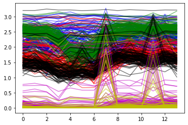
plt.plot(X_train[:,:14].T,'b',alpha=0.5)
plt.plot(X_train[:,14:14*2].T,'r',alpha=0.5)
plt.plot(X_train[:,2*14:14*3].T,'g',alpha=0.5)
plt.plot(X_train[:,3*14:14*4].T,'k',alpha=0.5)
plt.plot(X_train[:,4*14:14*5].T,'m',alpha=0.5)
plt.plot(X_train[:,5*14:14*6].T,'y',alpha=0.5)
plt.show()
ch_names = ['AF3','F7','F3','FC5','T7','P7','O1','O2','P8','T8','FC6','F4','F8','AF4']
bands = ['D_','T_','A_','B_','G1_','G2_']

feature_names = [[st+ch for ch in ch_names] for st in bands]
feature_names =  [f for flist in feature_names for f in flist]
#feature_names
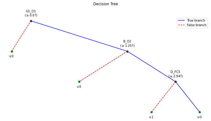
clf = ClassificationTree(max_depth=3)
clf.fit(X_train,y_train,feature_names=feature_names,verbose=1)
ytp = clf.predict(X_train)
ysp = clf.predict(X_test)

ytpr = clf.predict_proba(X_train)[:,1]
yspr = clf.predict_proba(X_test)[:,1]

print('Depth of trained Tree ', clf.getTreeDepth())
print('Accuracy')
print('- Training : ',np.mean(ytp==y_train))
print('- Testing  : ',np.mean(ysp==y_test))
print('Logloss')
Trloss = -np.mean(y_train*np.log(ytpr+1e-10)+(1-y_train)*np.log(1-ytpr+1e-10))
Tsloss = -np.mean(y_test*np.log(yspr+1e-10)+(1-y_test)*np.log(1-yspr+1e-10))
print('- Training : ',Trloss)
print('- Testing  : ',Tsloss)


plt.figure(figsize=(12,6))
clf.plotTree()
Number of features:: 84 Number of samples :: 100 ————————————— |Building the tree………………… |subtrees::|100%|——————–>|| |…………………….tree is buit! ————————————— Depth of trained Tree 3 Accuracy
- Training : 0.71
- Testing : 0.5681818181818182 Logloss
- Training : 0.5147251478695971
- Testing : 3.1215688661508283
Tuning ATAR
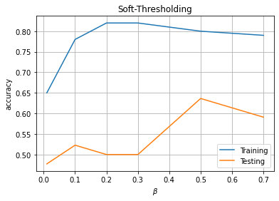
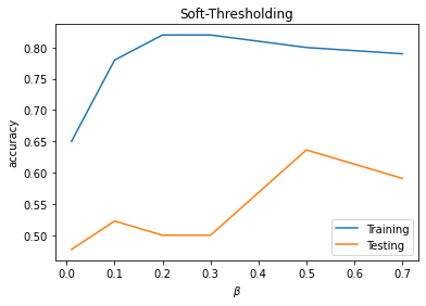
Soft-thresholding
PM1 = []
for beta in [0.01, 0.1,0.2, 0.3, 0.5, 0.7]:
print('='*50)
print('BETA = ',beta)
print('='*50)
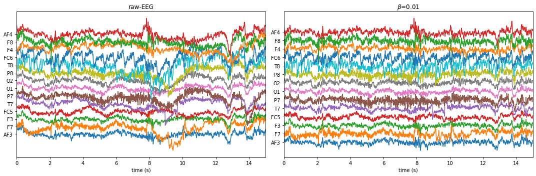
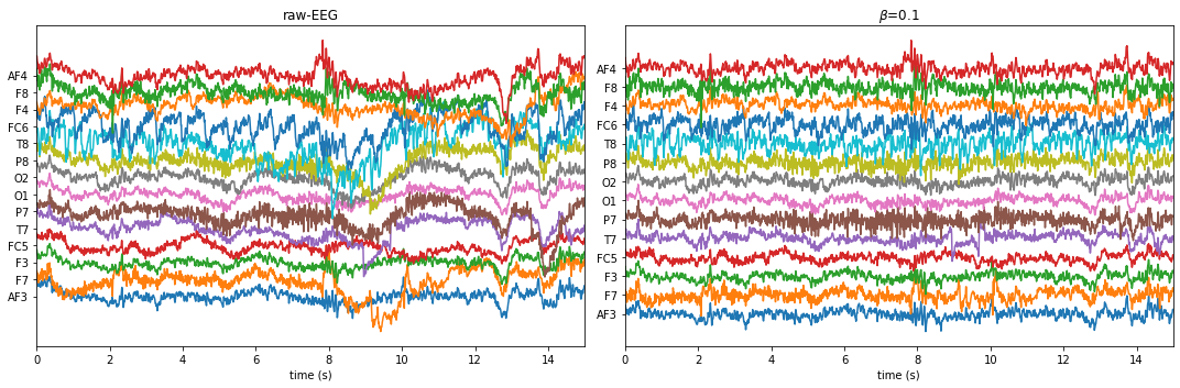
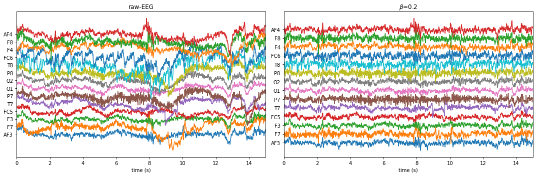
Subj.correct(method='ATAR',verbose=1,winsize=128*5,
wv='db3',thr_method='ipr',IPR=[25,75],beta=beta,k1=10,k2 =100,est_wmax=100,
OptMode ='soft',fs=128.0,use_joblib=False, useRaw=True)
X0 = Subj.getEEG(useRaw=True).to_numpy()[fs*20:fs*35]
X1 = Subj.getEEG(useRaw=False).to_numpy()[fs*20:fs*35]
t = np.arange(len(X0))/fs
plt.figure(figsize=(15,5))
plt.subplot(121)
plt.plot(t,X0 + np.arange(14)*50)
plt.xlim([t[0],t[-1]])
plt.xlabel('time (s)')
#plt.ylabel('amplitude')
plt.yticks(np.arange(14)*50,ch_names)
plt.title(fr'raw-EEG')
plt.subplot(122)
plt.plot(t,X1+ np.arange(14)*50)
plt.xlim([t[0],t[-1]])
plt.xlabel('time (s)')
#plt.ylabel('amplitude')
plt.yticks(np.arange(14)*50,ch_names)
plt.tight_layout()
plt.title(fr'$\beta$={beta}')
plt.show()
X_train,y_train,X_test, y_test = Subj.getXy_eeg(task=3, redo=True)
print('DataShape: ',X_train.shape,y_train.shape,X_test.shape, y_test.shape)
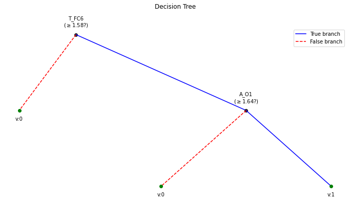
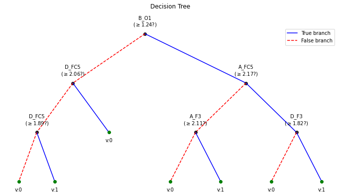
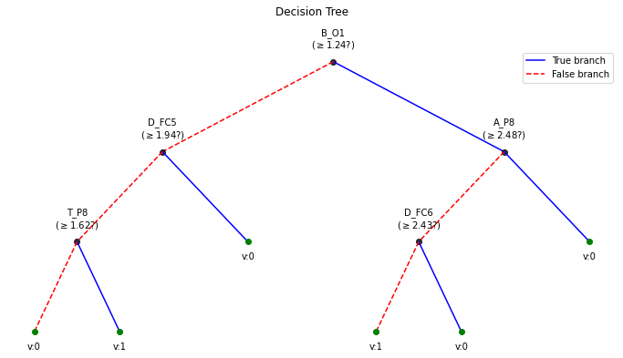
clf = ClassificationTree(max_depth=3)
clf.fit(X_train,y_train,feature_names=feature_names,verbose=1)
ytp = clf.predict(X_train)
ysp = clf.predict(X_test)
ytpr = clf.predict_proba(X_train)[:,1]
yspr = clf.predict_proba(X_test)[:,1]
print('Depth of trained Tree ', clf.getTreeDepth())
print('Accuracy')
print('- Training : ',np.mean(ytp==y_train))
print('- Testing : ',np.mean(ysp==y_test))
print('Logloss')
Trloss = -np.mean(y_train*np.log(ytpr+1e-10)+(1-y_train)*np.log(1-ytpr+1e-10))
Tsloss = -np.mean(y_test*np.log(yspr+1e-10)+(1-y_test)*np.log(1-yspr+1e-10))
print('- Training : ',Trloss)
print('- Testing : ',Tsloss)
plt.figure(figsize=(12,6))
clf.plotTree()
PM1.append([beta,np.mean(ytp==y_train),np.mean(ysp==y_test)])
print('='*50)
PM1 = np.array(PM1)
!==================================================
BETA = 0.01
!================================================== WPD Artifact Removal WPD: True Wavelet: db3 , Method: ipr , OptMode: soft IPR= [25, 75] , Beta: 0.01 , [k1,k2]= [10, 100] Reconstruction Method: custom , Window: [‘hamming’, True] , (Win,Overlap)= (640, 320)
If you are running feature extraction with DIFFERENT parameters again to recompute, set redo=True, else function will return pre-computed features, if exist
To suppress this warning2, set redo_warn=False
100%|##################################################|100\100|Sg - 0|
100%|##################################################|44\44|Sg - 0|
DataShape: (100, 84) (100,) (44, 84) (44,)
Number of features:: 84
Number of samples :: 100
—————————————
|Building the tree…………………
|subtrees::|100%|——————–>||
|…………………….tree is buit!
—————————————
Depth of trained Tree 2
Accuracy
- Training : 0.65
- Testing : 0.4772727272727273 Logloss
- Training : 0.5705223432488816
- Testing : 4.668722409182977
!==================================================
!==================================================
BETA = 0.1 !================================================== WPD Artifact Removal WPD: True Wavelet: db3 , Method: ipr , OptMode: soft IPR= [25, 75] , Beta: 0.1 , [k1,k2]= [10, 100] Reconstruction Method: custom , Window: [‘hamming’, True] , (Win,Overlap)= (640, 320)
If you are running feature extraction with DIFFERENT parameters again to recompute, set redo=True, else function will return pre-computed features, if exist
To suppress this warning2, set redo_warn=False
100%|##################################################|100\100|Sg - 0|
100%|##################################################|44\44|Sg - 0|
DataShape: (100, 84) (100,) (44, 84) (44,)
Number of features:: 84
Number of samples :: 100
—————————————
|Building the tree…………………
|subtrees::|100%|——————–>||
|…………………….tree is buit!
—————————————
Depth of trained Tree 3
Accuracy
- Training : 0.78
- Testing : 0.5227272727272727 Logloss
- Training : 0.3627270549616331
- Testing : 6.1363846139796685
!================================================== !================================================== BETA = 0.2 !================================================== WPD Artifact Removal WPD: True Wavelet: db3 , Method: ipr , OptMode: soft IPR= [25, 75] , Beta: 0.2 , [k1,k2]= [10, 100] Reconstruction Method: custom , Window: [‘hamming’, True] , (Win,Overlap)= (640, 320)
If you are running feature extraction with DIFFERENT parameters again to recompute, set redo=True, else function will return pre-computed features, if exist
To suppress this warning2, set redo_warn=False
100%|##################################################|100\100|Sg - 0|
100%|##################################################|44\44|Sg - 0|
DataShape: (100, 84) (100,) (44, 84) (44,)
Number of features:: 84
Number of samples :: 100
—————————————
|Building the tree…………………
|subtrees::|100%|——————–>||
|…………………….tree is buit!
—————————————
Depth of trained Tree 3
Accuracy
- Training : 0.82
- Testing : 0.5 Logloss
- Training : 0.3877860318279868
- Testing : 5.221099864589396
!================================================== !================================================== BETA = 0.3 !================================================== WPD Artifact Removal WPD: True Wavelet: db3 , Method: ipr , OptMode: soft IPR= [25, 75] , Beta: 0.3 , [k1,k2]= [10, 100] Reconstruction Method: custom , Window: [‘hamming’, True] , (Win,Overlap)= (640, 320)
plt.plot(PM1[:,0],PM1[:,1],label='Training')
plt.plot(PM1[:,0],PM1[:,2],label='Testing')
plt.xlabel(r'$\beta$')
plt.ylabel('accuracy')
plt.title('Soft-Thresholding')
plt.legend()
plt.show()
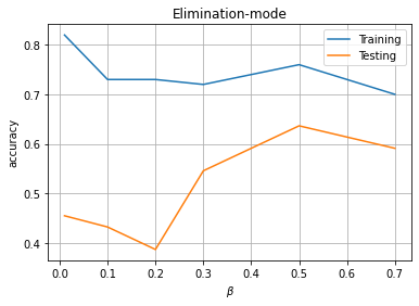
Elimination mode
PM2 = []
for beta in [0.01, 0.1,0.2, 0.3, 0.5, 0.7]:
    print('='*50)
    print('BETA = ',beta)
    print('='*50)
    Subj.correct(method='ATAR',verbose=1,winsize=128*5,
            wv='db3',thr_method='ipr',IPR=[25,75],beta=beta,k1=10,k2 =100,est_wmax=100,
            OptMode ='elim',fs=128.0,use_joblib=False, useRaw=True)

    X0 = Subj.getEEG(useRaw=True).to_numpy()[fs*20:fs*35]
    X1 = Subj.getEEG(useRaw=False).to_numpy()[fs*20:fs*35]
    t = np.arange(len(X0))/fs

    plt.figure(figsize=(15,5))
    plt.subplot(121)
    plt.plot(t,X0 + np.arange(14)*50)
    plt.xlim([t[0],t[-1]])
    plt.xlabel('time (s)')
    #plt.ylabel('amplitude')
    plt.yticks(np.arange(14)*50,ch_names)
    plt.title(fr'raw-EEG')
    plt.subplot(122)
    plt.plot(t,X1+ np.arange(14)*50)
    plt.xlim([t[0],t[-1]])
    plt.xlabel('time (s)')
    #plt.ylabel('amplitude')
    plt.yticks(np.arange(14)*50,ch_names)
    plt.tight_layout()
    plt.title(fr'$\beta$={beta}')
    plt.show()


    X_train,y_train,X_test, y_test = Subj.getXy_eeg(task=3, redo=True)

    print('DataShape: ',X_train.shape,y_train.shape,X_test.shape, y_test.shape)


    clf = ClassificationTree(max_depth=3)
    clf.fit(X_train,y_train,feature_names=feature_names,verbose=1)
    ytp = clf.predict(X_train)
    ysp = clf.predict(X_test)

    ytpr = clf.predict_proba(X_train)[:,1]
    yspr = clf.predict_proba(X_test)[:,1]

    print('Depth of trained Tree ', clf.getTreeDepth())
    print('Accuracy')
    print('- Training : ',np.mean(ytp==y_train))
    print('- Testing  : ',np.mean(ysp==y_test))
    print('Logloss')
    Trloss = -np.mean(y_train*np.log(ytpr+1e-10)+(1-y_train)*np.log(1-ytpr+1e-10))
    Tsloss = -np.mean(y_test*np.log(yspr+1e-10)+(1-y_test)*np.log(1-yspr+1e-10))
    print('- Training : ',Trloss)
    print('- Testing  : ',Tsloss)


    plt.figure(figsize=(12,6))
    clf.plotTree()

    PM2.append([beta,np.mean(ytp==y_train),np.mean(ysp==y_test)])

    print('='*50)

PM2 = np.array(PM2)